Neural Network Basics

Classification problem

There are various applications of neural-network models. In this section, for simplicity of discussion, we will focus only on the classification problem. In the classification problem, when the number of output classes is \(V\), then the class index \(v\) may take a value in the following range:

(1)\[ 0 \le v \le V - 1.\]

In stead of the above sparse representation of the output class, we may use the one-hot vector representation as below:

Sometimes, the class index \(v\) in (1) is referred to as sparse representation compared to the one-hot vector representation in Table

Model

In the classification problem, the model can be considered a function to predict the output class probability \(\bsf{y}\) given the input \(\bsf{x}\). Thus when the model is represented by a function \(f\), the relation is represented by the following equation.

(2)\[ \hat{\bsf{y}} = f\left(\bsf{x}\right)\]

Training Data Set

In this section, we consider the supervised training case, which might be the most basic case of training neural-network models. Other cases such as unsupervised or semi-supervised training cases will be covered later.

(3)\[ \mathcal{T} = \big \{ (\bsf{x}^{(k)},\, \bsf{y}^{(k)}) \; \big | \; 0 \le k \le N_{\text{tr}} - 1 \big \},\]

where \(N_{\text{tr}}\) is the number of examples in the training set \(\mathcal{T}\).

Loss Function

In training neural network models, our objective is making the model output \(\hat{\bsf{y}}\) as close to the ground truth \(\bsf{y}\) as possible. To perform this task analytically, we usually define a certain loss function and minimize it.

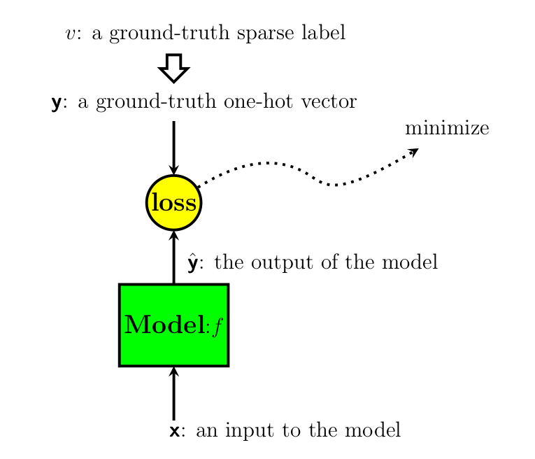
Fig. 1 A model and the corresponding loss.

The entire loss \(\mathbb{L}\) is defined by the following equation for the entire training set defined in (3):

(4)\[ \mathbb{L} = \frac{1}{N_{\text{tr}}} \sum_{k=0}^{N_{\text{tr} - 1}} \text{loss}(\bsf{y}^{(k)}, \hat{\bsf{y}}^{(k)}) \]

where \(N_{tr}\) is the number of training examples as defined in

Now, the question is what would be a good candidate for the loss function in (4). Various types of functions may be condidates for this loss function including the well know \(L_1\) or \(L_2\) losses and so on. As will be discussed later, an appropriate loss function is different depending on applications.

In the classification problem, we would like to make the distribution of prediction by the model \(\hat{\bsf{y}} = f(\bsf{x})\) as close to the distribution of the training data set as possible. In this classification problem, note that both the ground truth output \(\bsf{y}\) and the predicted output \(\hat{\bsf{y}}\) are probability distributions of the set of output labels defined in (1).

To measure the difference between two distributions, we may use the KL divergence or the Cross Entropy (CE). Since the distribution of the training set is already fixed, minimizing the following Cross Entropy (CE) loss is equvalent to minizing the KL divergence, which is shown in the following equation:

\[\begin{split} \mathbb{L}_{\text{CE}} & = H(\bsf{y}, \bsf{\hat{y}}) \\ & = H(\bsf{y}) + D_{\text{KL}} (\bsf{y} || \hat{\bsf{y}})\end{split}\]

From the definition of cross entropy (CE), \(\mathbb{L}_{\text{CE}}\) is given by the following equation:

(5)\[\begin{split} \mathbb{L}_{\text{CE}} & = -E_{\bsf{y} \sim \text{training_data}} \left[ \log \hat{\bsf{y}} \right]. \\\end{split}\]

When the one-hot vector representation is used in (5), (5) is calculated as follows:

(6)\[\begin{split} \mathbb{L}_{\text{CE}} & = -E_{\bsf{y} \sim \text{training_data}} \left[ \sum_{v=0}^{V-1} y_v \log \hat{y}_v \right]. \\\end{split}\]

where \(y_v\) and \(\hat{y}_v\) are \(v\)-th element of the one-hot vector \(\mathbf{y}\) and \(\hat{\mathbf{y}}\) respectively, and \(V\) is the number of output classes as shown in (1).

(6) may be expressed in summation rather than the expection as follows:

(7)\[\begin{split} \mathbb{L}_{\text{CE}} & = -\sum_{k=0}^{N_{\text{tr}}} \sum_{v=0}^{V-1} y^{(k)}_v \log \hat{y}^{(k)}_v . \\\end{split}\]

where \(y^{(k)}_v\) and \(\hat{y}^{(k)}_v\) represent the \(v\)-th element of the one-hot vector of the k-th training example \(\mathbf{y}^{(k)}\) and the corresponding predicted output using the model \(\hat{\mathbf{y}}^{(k)}\).

In Tensorflow, cross entropy is calculated using tf.nn.softmax_cross_entropy_with_logits for one hot vector representation and tf.nn.sparse_softmax_cross_entropy_with_logits for sparse matrix representation.

Softmax and Logit

For classification tasks, we usually apply the softamx function to represent the probabilities corresponding to each class.

(8)\[ Softmax(\mathbf{h})_j = \frac{\exp(h_j)}{\sum_{i=0}^{C-1} \exp(h_i)}\]

Gradient Descent

Suppose that the entire parameters of our neural network model is denoted by \(\mathsf{w}\). If we can directly differentiate the loss function \(\mathbb{L}\), we improve the model parameters using the well-known Gradient Descent approach as shown below:

(9)\[\begin{align} \bsf{w} \leftarrow \bsf{w} - \mu \nabla_{\bsf{w}} \mathbb{L}. \end{align}\]

where \(\mu\) is a constant called the learning rate.

It is well known that the direction of the negative of gradient is the direction of steepest descent in the surface defined by the loss function \(\mathbb{L}\). However, Gradient Descent (GD) is not a practical approach when the training set size is sufficiently large for the following two reasons.

• Inefficiency in computation
  It is usually not possible to load all the training examples in memory at once. Thus, we may need to store partial results and part of inputs in the disk, and repeatedly load and save partial result.

• Slow convergence
  Parameter update is done only once after processing the entire training set. That is to say, the parameter update is done only once for one epoch.

Stochastic Gradient Descent (SGD)

Unlike the GD approach using the loss from the entire training dataset, in SGD, we update the parameter for each training example \((\bsf{x}^{(k)}, \bsf{y}^{(k)})\) iteratively.

(10)\[\begin{align} \bsf{w} \leftarrow \bsf{w} - \mu \nabla_{\bsf{w}} \mathbb{L}^{(k)} \end{align}\]

where \(\mathbb{L}^{(k)}\) is the loss value calculated using only a single training example \((\bsf{x}^{(k)}, \bsf{y}^{(k)})\) and the prediction by the model \(\hat{\bsf{y}}^{(k)}\):

\[ \mathbb{L}^{(k)} = \text{loss}(\bsf{y}^{(k)}, \hat{\bsf{y}}^{(k)})\]

Back-Propagation

Questions

Q1. Calculate the cross entropy between the following two vectors containing probability distributions:

Q2.